Table of Contents
Mapping and assessment
Spatial analysis of Ecosystem Services
Spatial data analysis1) is an ensemble of techniques which study entities characterized by a precise location in space. It is commonly applied to geographic information. Georeferenced in the sense that they are typically structured as a combination of attributes (the feature associate to a given location) and a couple of values, i.e. the coordinates, identifying the location within a recognized Reference System (e.g. WGS84, UTM, etc.)
Spatial analysis includes a variety of techniques, developed to derive quantitative indicators as outcomes of algorithms applied to spatial data and in particular to their topological, geometric, or geographic properties. The algorithms are typically applied to raster based GIS layers, for example by means of spatial convolution indices, calculating descriptive context statistics by means of moving windows across the study area.
In the case of spatial analysis applied to ES, examples are:
- Cost analysis performed by calculating a proximity (or cost) surface over a friction map, e.g. to map the potential fruition of recreational areas by tourists, or the ecological connectiveness by analysing corridors between habitats.
- Visibility analysis of landscapes, to determine all areas that can be seen from one or more viewpoints, to determine the recreational values.
- Analysis of watersheds, with calculation of slope, water accumulation, etc., to determine the potential benefit deriving from the protection of upstream land.
- Spatial models, such as plant (e.g. crop) productivity for the calculation of provisioning services.
Spatial analyses for the assessment of ESs are typically designed as a sequence of steps applied to input maps in a logical sequence, to produce intermediate and output layers, which are typically maps of supply, flow and demand of ES2).
ES Spatial Analysis in the AlpES Project
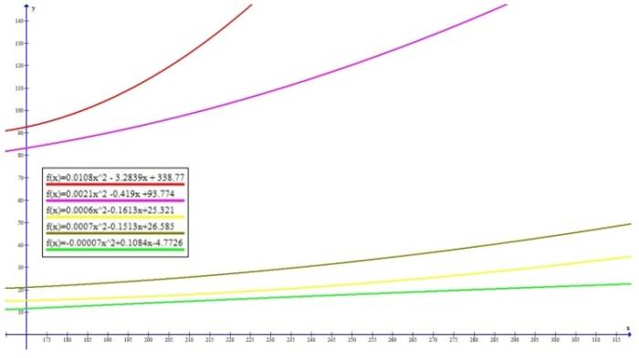
Biomass production for livestock uses is an ES that strictly depends on local climate and biophysical parameters. Either these spatial data are collected from local institutions or indirectly obtained from remote sensing (RM), they can be used to estimate potential productivity of pastures and grasslands. In the AlpES project, statistical models are applied to quantify kg of production in dry matter per hectare, depending on the length of the growing season. The growing season is a typical proxy used to define the number of vegetation days i.e. the days in which the temperature is sufficiently high to induce biomass accumulation through synthesis of new plant tissues. For fodder production the temperature threshold was set to 5° C. Graph 1 reports the statistical models used to estimate biomass production. These models can be implemented by using simple map algebra tools, usually available in any GIS software, like QGIS and ArcGIS. A vigor factor (VF) has been assigned to each land cover as local productivity is assumed to be different depending on the specific land cover class: for example, alpine pastures have clearly higher biomass productivity compared to moors and heathland. Consequently, different growth curves have been chosen to estimate biomass growth based on the raster map that displays the number of vegetation days per cell.
<font 11px/inherit;;inherit;;inherit>Graph 1. Biomass growth curves: VF 5 (red); VF4 (purple); VF 3 (yellow); VF 2 (dark green); VF 1 (light green). The x-axis reports the number of vegetation days. The y-axis reports the biomass productivity in deci-tons of dry mass per hectare (EURAC).</font>
In general, land cover data are often used to quantify spatially explicit indicators of ES supply3).
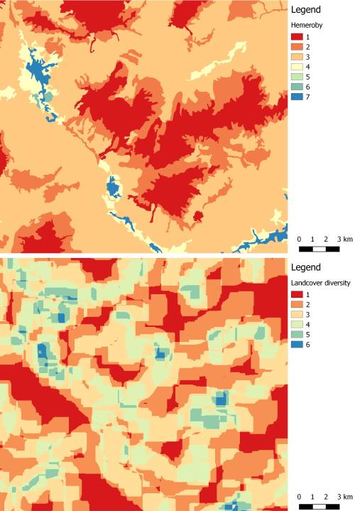
An example is the hemeroby index i.e. the degree of human influence. It is based on Paracchini and Capitani (2011)4) who have classified the degree of human influence in a decreasing ranking (7 to 1), by matching ranks to each class of Corine Land Cover (CLC) classification. For example, urban areas are assumed to be low providers of recreational activities (hemeroby index 7) while forests offer several opportunities for outdoor leisure and to practice sports (hemeroby index 2, 3 or 4). Thus, within AlpES project, hemeroby indexes have been derived through the reclassification of CLC codes, as indicator of the ES “outdoor recreation activities” (Figure 1).
For the same ES, another example is the diversity of landcover, which is based on the assumption that spatial heterogeneity provides high recreational and visual attractiveness5). The spatial analysis is carried out by iterating a moving window of a defined shape on every pixel of the landcover map. The number of landcover types can be counted in the surrounding cells and recorded within each pixel, representing the landcover heterogeneity that can be observed in the neighborhoods. In AlpES project, a moving window of 1 km per side has been used to calculate landcover diversity (Figure 1).
<font 11px/inherit;;inherit;;inherit>Figure 1. Detail of pilot region LAG Alto Bellunese: hemeroby index, where value close to 1 implies a low degree of human influence (top); number of different landcover types per km² (bottom).</font>
Accessibility is the proxy of the degree to which people can actually benefit from high recreation potentials6). In AlpES project, accessibility has been calculated by means of a cost-distance algorithm7) 8), which determines the cumulative cost of moving to each cell on a cost surface map, from other user-specified geographic coordinates (e.g. the coordinates of the centroids of polygons representing urban areas). Each cell in the input cost map contains a value that represents the cost of moving from that cell to its neighbors. The output map displays the least cost path from each pixel of the cost surface to closest urban areas, extracted from the landcover map (CLC codes 111, 112). To quantify accessibility the cost was expressed in term of travel time.
Whenever an ES is estimated through a portfolio of indicators, a spatial multi-criteria analysis (MCAs) can be applied. For example, this approach has been helpful to display recreation potential hotspots in a relative and easy-to-read manner. In MCA, worth to be mentioned are the steps of normalization and aggregation:
• normalization9) is a method used to convert data variability in a common numerical scale (0 to 1 or 0 to 100 %);
• once all indicators share a common scale, they can be aggregated in a single meaningful value that is defined by the “contribution” of each indicator to the final estimation of the ES; this contribution can be equal or weighted depending on stakeholder preference structure10).
All normalization and aggregation procedures can be easily implemented with map algebra tools of any GIS software.
Recreation supply has to be compared with demand for outdoor activities by using demographic data and available information on tourism overnight stays. Demography, tourism and other data referred to municipalities or different administrative levels (NUTS and LAU) are typically available in vector formats (e.g. ESRI shapefile). In this case, elaborations are carried out in spatial databases connected to IDs of each geometry (points, lines of polygons). Among others, selection of records, creation of attributes and calculations are GIS tasks performed using software-specific expression to manipulate databases and geometries. For example, the potential demand for outdoor recreation activities has been estimated by calculating the “permanent resident equivalents” of tourism occupancy11). In the field calculator of QGIS, the code “PRES”/365+“POP” apply the equation to all records (municipality) of each attribute, whose names are written between quotations. “PRES” represents the sum of overnight stays for all tourists in the period of 1 year. “POP” represents population data. A new attribute is therefore created, reporting “permanent resident equivalents” per municipality.
Additional Resources
Examples of applications:
- PEER Spatial Assessment: http://www.peer.eu/fileadmin/user_upload/publications/PEER_report_4_phase_2.pdf
- Global Forest Watch: http://www.globalforestwatch.org/howto/gis/gis-spatial-analysis-in-qgis.html
- ESP Visualization tool (ESP-VT): http://esp-mapping.net/Home/
Examples of tools:
- QGIS Plugins for spatial analysis: https://plugins.qgis.org/plugins/

